Statistical Consultants Ltd |
      |
Benford's Law ExplainedStatistical Theory, Accounting, Forensics / Fraud Detection Date posted: This post continues from the previous post: Benford’s Law and Accounting Fraud Detection. There are several ways of explaining why Benford’s law works, including the following: Multiplying DistributionsBenford’s distribution becomes more prominent when data is taken from a mixture of several distributions, with values from those distributions multiplied together, resulting in right skewed data. In accounting, the types of data which often conform to Benford’s Law involve a multiplication of two variables i.e. prices multiplied by quantities. Theorem: Let X be a random variable with a continuous probability density function. There exists  such
that for all
such
that for all  : : conforms
to Benford’s Law (for any value of scaling
parameter conforms
to Benford’s Law (for any value of scaling
parameter  ) )The following animated gif shows a distribution and its corresponding first digit distribution as the exponent used to transform the data increases. The data happens to be 10,000 observations randomly generated from a normal distribution of mean 100 and standard deviation 10.  Exponential Growth ProcessesThis explanation is similar to the explanation for the rank-size rule of city populations. For many data sets that conforms to Benford’s Law (especially accounting data due to inflation, money supply expansion, interest etc), the figures tend to follow Gibrat’s law of proportional growth i.e. the figures grow by amounts proportional to the size of the current figure. Over time, a variable (such as a reoccurring expense) would spend more of its time with lower first digits, than higher first digits. For example, lets say the variable x starts with a value of 10. The variable would spend more time being:  than
than  and more time being:
than  … and so on. Once the variable reaches the hundreds, it would spend more time being:  than
than  and more time being:
than  … and so on. Overall, lower first digits would be more common than the higher first digits. Scale InvarianceWhile the previous explanations show what kind of data would conform to Benford’s Law (and how it comes about), scale invariance explains how the formula for Benford’s distribution can be derived. If the first digits of some large data set conform to a particular distribution, then the distribution should be independent of the data’s units of measurement. For example, changing the units of measurement from dollars to yen shouldn’t change the distribution of digits (it would likely change many individual first digits but not their overall distribution). Rough Derivation: Let’s say that x has a scale invariant distribution. If x is scale invariant then: 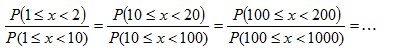 This can make the derivation simpler by allowing the assumption that:  If x is scale invariant, then multiplying x by a constant won’t change its distribution. Multiplying x by a constant, is equivalent of adding a constant to log(x). Since x is scale invariant, then adding a constant to log(x) wouldn’t change the distribution of log(x). The only probability distribution that doesn’t change when a constant is added, is the uniform distribution. This would mean: 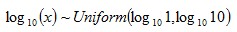 Therefore:  Since
and ,
then: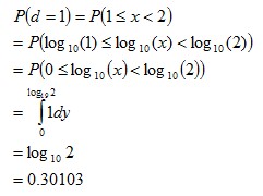 where  Or more generally: 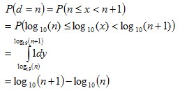 where See also:Benford’s Law and Accounting Fraud DetectionThe Rank-Size Rule of City Populations |
|
|
| Copyright © Statistical Consultants Ltd 2011 |