Statistical Consultants Ltd

The Rank-Size Rule of City Populations

Geography, Statistical Theory, Data Tables, Statistical Modelling

Date posted: 22 March 2011

The rank-size rule (or rank-size distribution) of city populations, is a commonly observed statistical relationship between the population sizes and population ranks of a nation’s cities. For many years, the reasoning behind the rank-size rule was unknown (at least to geographers).

In its most restrictive form (as devised by geographers), the rule is:
rank-size rule (restrictive form)

where:
x is the rank of the city’s population i.e. a 1 for the highest population, 2 for the second highest etc.

is the population size of the city ranked x

is the population size of the largest city

The rule can be loosened to the following:
rank-size rule (loosened form)

where A and b are parameters that don’t necessarily conform to

and 1 respectively.

The rank-size rule is a multiplicative relationship (hyperbola / curved) and when graphed, is convex to the origin. The relationship isn’t linear, nor is it concave to the origin.

The relationship is multiplicative and convex to the origin.

The relationship is multiplicative and convex to the origin.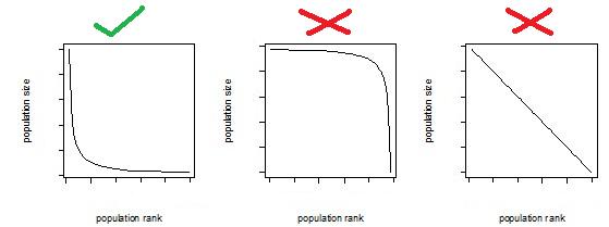

The loosened form of the equation fits better to real data, than its original restricted form. The loosened form of the equation usually fits very well to real rank-size data of a nation’s cities. The loosened form of the equation can be rewritten as follows: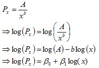

rank-size rule (rearranged)

The equation in the final row can be fitted easily using regression (double-log model).

The Rank-Size Distribution of US Cities

The following data set is of the 2009 population sizes and ranks of USA’s 276 biggest cities:

USAcities2009.csv

When plotting the population sizes and ranks, the two variables appear to have a strong multiplicative relationship.

graph of multiplicative relationship

When plotting the logs of the two variables, it makes the multiplicative relationship even more obvious.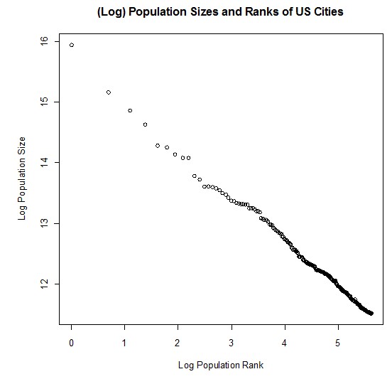

graph of double-logged variables

A double-log model (as described earlier) was fitted to the data via regression. The following regression output was obtained:

Call:
lm(formula = log(Population) ~ log(Rank))

Residuals:
     Min       1Q   Median       3Q      Max
-0.21820 -0.01990 -0.00368 0.02279 0.26833

Coefficients:
             Estimate Std. Error t value Pr(>|t|)
(Intercept) 15.674447   0.013896 1128.0   <2e-16 ***
log(Rank)   -0.742429   0.002936 -252.9   <2e-16 ***
---
Signif. codes: 0 ‘***’ 0.001 ‘**’ 0.01 ‘*’ 0.05 ‘.’ 0.1 ‘ ’ 1

Residual standard error: 0.04691 on 274 degrees of freedom
Multiple R-squared: 0.9957,     Adjusted R-squared: 0.9957
F-statistic: 6.394e+04 on 1 and 274 DF, p-value: < 2.2e-16

For those who aren’t familiar with regression output:

The very high (close to one) R-squared statistic shows that the model fits very strongly to the data:

Multiple R-squared: 0.9957

The very low (close to zero) p-values of the t-values, show that the parameters of the model are highly significant:

Pr(>|t|)
<2e-16 ***
<2e-16 ***

The coefficient estimates replace the unknown parameters, and the equation can then be rearranged to be in the form of the rank-size rule formula shown earlier.

             Estimate
(Intercept) 15.674447
log(Rank)   -0.742429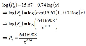

regression output equation rearranged

Reasons for the Rank-Size Rule

According to The Dictionary of Human Geography published in 1986 (ISBN 0 631 14656 3):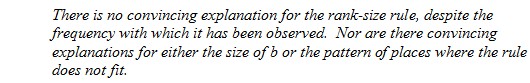

dictionary statement

For many years, the reasoning behind the rank-size rule was unknown (at least to geographers). Some geographers gave some plausible but weak reasons (based around economic and geographical theories) for why it might occur. The reason why the rank-size rule is so common and strong is due to statistical/mathematical reasons.

In short, the rank-size rule occurs because:

The relationship between population size and population rank is inherently negative. This is obvious and accounts for much of the strong fit, but alone doesn’t account for the multiplicative and convex (to the origin) relationship.
Growth rates are independent of city size (or at least weakly related) and absolute growth is roughly proportional to city size. This is known as Gibrat’s Law or Gibrat’s rule of proportional growth. For example, a city grows on average at a rate of 1% per year, regardless of the city’s size.
The growth rates between cities aren’t equal. The growth rates within cities also vary over time, but some cities would on average grow faster than others.

Gibrat’s law and the unequal growth rates, lead to a strengthening of the multiplicative relationship over time. In the long run, a multiplicative convex (to the origin) relationship would develop even if the initial relationship was linear or multiplicative but concave to the origin, or if the initial population sizes were equal.

The following animated gifs show simulated rank-size distributions changing over time. Each example has a different starting distribution (linear, constant or concave to the origin), and each observation within an example is randomly assigned a growth rate. At each step of the simulation, a unit of time passes, and the populations of each city grow proportionately by their assigned growth rate. The rankings change if one city’s population overtakes another.

Example 1: Initial Relationship is Linear

Simulation of rank-size over time (initial relationship is linear)

Simulation of rank-size over time (initial relationship is linear)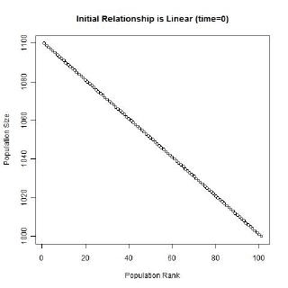

Example 2: Initial Population Sizes are Equal

Simulation of rank-size over time (initial population sizes are equal)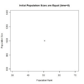

Example 3: Initial Relationship is Concave to the Origin

Simulation of rank-size over time (initial relationship is concave)

Statistical Consultants Ltd

The Rank-Size Rule of City Populations

The Rank-Size Distribution of US Cities

Reasons for the Rank-Size Rule

See also: